Introduction
A while back (around May 2025) I got interested in thermal performance curves after seeing several interesting presentations at a SEEC symposium by students of Prof. Susana Clusella-Trullas’s. One student had fit a plethora of models, both convenetional and otherwise, and found it difficult to decide which was “best”. Much reference was made to a paper claiming that there was no “one size fits all” model for this sort of data (https://www.nature.com/articles/s41467-024-53046-2).
Background
A bit of background: thermal performance curves (TPCs) are descriptions of how well organisms perform under a range of temperatures. This is usually assessed experimentally (though in some cases one could use observational data). Performance is a relatively vague concept, but it is intended to serve as an indicator of fitness potential. As such, it can be measured in a number of ways, many of which are particular to the organism under study, and most of which are some kind of rate. In plants, one might measure growth or photosynthetic rate; in bacteria, one might measure colony growth; in animals, movement speed and metabolic rate are frequently used.
It occurred to me that many TPC experiments produce data with a hierarchical structure. For example, in many cases the same individual is measured across the full range of assay temperatures. In other instances, one might have several blocks representing each temperature treatment, with a number of individuals measured in each. Such structure should be taken into account when modelling. To my surprise, however, according to my (admittedly somewhat shallow) research, this did not appear to be the norm. Instead, when multiple measurements are taken per individual the standard approach appears to be to fit a separate model to each individual and discard individuals with “too few data points” or for which the model fails to converge. And when individuals are only measured once but multiple individuals are measured per treatment, their performance values are often averaged as a way of accounting for uneven sampling effort.
Many mathematical models have been proposed to describe the types of TPCs typically encountered. Most of them follow the same basic form: at low temperatures, performance is poor; then, it ramps up exponentially, plateauing just before reaching a peak; finally performance takes a nose-dive, steeply dropping before reaching zero at the critical upper thermal limit. In the paper I mentioned above, Kontopoulos et al. fit 83 of these models to each of 2,739 TPC data sets and found that none of the models consistently outperformed the others. Many if not most of these models are implemented in the comprehensive and widely used R package rTPC (https://padpadpadpad.github.io/rTPC/reference/index.html), whose documentation includes a number of vignettes on using the rTPC functions alongside the nls.multstart package for model fitting by maximum likelihood. One thing that’s missing is mention of how to explicitly account for the hierarchical nature of many TPC data sets. Instead, recommendations for such data include, for example, i) fitting TPCs independently to each individual when the same individual is measured across the full range of assay temperatures (here); ii) using the mean for each temperature but using inverse standard deviation weighting to account for measurement error (https://padpadpadpad.github.io/rTPC/articles/model_weighting.html); and iii) complicated bootstrapping methods to approximate uncertainty intervals (https://padpadpadpad.github.io/rTPC/articles/weighted_bootstrapping.html).
I strongly suspected that a Bayesian hierarchical approach could do all of these things much more elegantly. To test this idea, I tried to replicate some of the examples presented in the rTPC vignettes in a Bayesian framework, and then adapt them to the hierarchical way of doing things. I used the brilliant brms R package for all my model specification, fitting (using Stan), and post-processing needs. This package makes all of these things easy, and its straightforward syntax for non-linear formulae and prior specifications came in particularly clutch.
1
2
3
| set.seed(42)
library(rTPC)
library(tidyverse)
|
1
2
3
4
5
6
7
8
9
10
| ## ── Attaching core tidyverse packages ──────────────────────── tidyverse 2.0.0 ──
## ✔ dplyr 1.1.4 ✔ readr 2.1.6
## ✔ forcats 1.0.1 ✔ stringr 1.6.0
## ✔ ggplot2 4.0.1 ✔ tibble 3.3.0
## ✔ lubridate 1.9.4 ✔ tidyr 1.3.1
## ✔ purrr 1.2.0
## ── Conflicts ────────────────────────────────────────── tidyverse_conflicts() ──
## ✖ dplyr::filter() masks stats::filter()
## ✖ dplyr::lag() masks stats::lag()
## ℹ Use the conflicted package (<http://conflicted.r-lib.org/>) to force all conflicts to become errors
|
1
2
3
4
5
| library(ggrepel)
theme_set(theme_bw())
# Prepare for Stan and brms
library(brms)
|
1
2
3
4
5
6
7
8
9
10
| ## Loading required package: Rcpp
## Loading 'brms' package (version 2.23.0). Useful instructions
## can be found by typing help('brms'). A more detailed introduction
## to the package is available through vignette('brms_overview').
##
## Attaching package: 'brms'
##
## The following object is masked from 'package:stats':
##
## ar
|
1
2
3
| options(brms.backend = "cmdstanr")
library(marginaleffects) # for convenient predictions
library(ggdist)
|
1
2
3
4
5
6
| ##
## Attaching package: 'ggdist'
##
## The following objects are masked from 'package:brms':
##
## dstudent_t, pstudent_t, qstudent_t, rstudent_t
|
1
2
3
4
5
6
| ##
## Attaching package: 'tidybayes'
##
## The following objects are masked from 'package:brms':
##
## dstudent_t, pstudent_t, qstudent_t, rstudent_t
|
The data
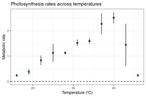
The chlorella_tpc data are heavily referenced in the rTPC docs and conveniently have a clear hierarchical structure, with multiple temperature assays per algal colony. This is a dataset of 60 TPCs of respiration and photosynthesis of the aquatic algae, Chlorella vulgaris. The colonies were grown at different temperatures for two lengths of time (~10 generations = “acclimation”, ~100 generations = “adaptation”)
Measurement error method
I’ll start by reimplementing the weighted samples approach presented here. brms allows us to do this with resp_se. I’ll also switch to the Pawar et al. (2018) model, as the model in the vignette has three parameters with no biological meaning, which complicates prior specification. The pawar_2018 model has five parameters: $t_{ref}$ is an “anchor” parameter that is fixed, being the temperature at which the $r_{tref}$ rate is estimated. $t_{ref}$ should be below $t_{opt}$, the temperature at which the rate peaks. That rate is informed by the activation energy $e$ and the deactivation energy $eh$, which control the rate of incline and decline. $e$ cannot be greater than $eh$. The rTPC::get_start_vals() function is a convenient way to get an idea of plausible values for these parameters.
Here is the model equation:
\[\mathrm{rate} = \frac{r_{\mathrm{tref}}\; \exp\!\Bigl(\!-\frac{e}{k}\bigl(\frac{1}{T + 273.15} - \frac{1}{T_{\mathrm{ref}} + 273.15}\bigr)\Bigr)} {1 + \bigl(\frac{e}{e_h - e}\bigr)\; \exp\!\Bigl(\frac{e_h}{k}\bigl(\frac{1}{T_{\mathrm{opt}} + 273.15} - \frac{1}{T + 273.15}\bigr)\Bigr)}\]
First, let’s fit the ML model.
1
2
3
4
5
6
7
8
9
10
11
12
13
14
15
16
17
18
19
20
21
22
23
24
25
26
27
28
29
30
31
32
33
| ## get curve data
data("chlorella_tpc")
d_ave <- filter(
chlorella_tpc,
process == 'adaptation',
growth_temp == 33,
# our rate will be the metabolic rate of photosynthesis
flux == 'photosynthesis'
) %>%
group_by(temp) %>%
# Get the average, SD, and SE
summarise(
.,
sd = sd(rate),
ave_rate = mean(rate),
n = n(),
se = sd / sqrt(n)
) %>%
ungroup()
# plot
ggplot() +
geom_linerange(aes(x = temp, ymin = ave_rate - sd, ymax = ave_rate + sd), d_ave) +
geom_point(aes(temp, ave_rate), d_ave, size = 2, shape = 21, fill = 'green4') +
theme_bw(base_size = 12) +
theme(legend.position = 'none',
strip.text = element_text(hjust = 0),
strip.background = element_blank()) +
labs(x ='Temperature (ºC)',
y = 'Metabolic rate',
title = 'Photosynthesis rates across temperatures') +
geom_hline(aes(yintercept = 0), linetype = 2)
|
1
2
3
4
5
6
7
8
9
10
11
12
13
14
15
16
17
18
19
20
21
22
23
24
25
| # Fit with nls.multstart
ml_model_weighted <- nls.multstart::nls_multstart(
ave_rate ~ pawar_2018(temp = temp, rtref, e, eh, topt, tref = 20),
data = d_ave,
iter = c(4, 4, 4, 4),
start_lower = get_start_vals(
d_ave$temp,
d_ave$ave_rate,
model_name = 'pawar_2018'
) -
10,
start_upper = get_start_vals(
d_ave$temp,
d_ave$ave_rate,
model_name = 'pawar_2018'
) +
10,
lower = get_lower_lims(d_ave$temp, d_ave$ave_rate, model_name = 'pawar_2018'),
upper = get_upper_lims(d_ave$temp, d_ave$ave_rate, model_name = 'pawar_2018'),
supp_errors = 'Y',
convergence_count = FALSE,
# include weights here!
modelweights = 1 / sd
)
summary(ml_model_weighted)
|
1
2
3
4
5
6
7
8
9
10
11
12
13
14
15
16
| ##
## Formula: ave_rate ~ pawar_2018(temp = temp, rtref, e, eh, topt, tref = 20)
##
## Parameters:
## Estimate Std. Error t value Pr(>|t|)
## rtref 0.52846 0.06160 8.579 5.82e-05 ***
## e 0.66967 0.07411 9.036 4.16e-05 ***
## eh 7.01783 1.38740 5.058 0.00147 **
## topt 39.70098 0.78126 50.817 2.99e-10 ***
## ---
## Signif. codes: 0 '***' 0.001 '**' 0.01 '*' 0.05 '.' 0.1 ' ' 1
##
## Residual standard error: 0.4537 on 7 degrees of freedom
##
## Number of iterations to convergence: 24
## Achieved convergence tolerance: 1.49e-08
|
Fit the Bayesian version.
We need to do some preparation first in order to export the pawar_2018() funtion to brms.
1
2
3
4
5
6
7
8
9
10
11
12
13
14
15
16
17
18
19
20
21
22
23
24
25
26
27
28
29
30
31
32
33
34
35
36
37
38
39
40
41
42
43
44
45
46
47
48
49
50
51
52
53
54
55
56
57
58
59
60
61
62
63
64
65
66
67
68
69
70
71
72
73
74
75
76
77
78
79
80
81
82
83
84
85
86
87
88
89
| pawar_2018a <- function(temp, r_tref, e, eh, topt) {
Z <- 273.15 # Absolute zero
tref <- 20
tref <- Z + tref
k <- 8.617e-05 # The boltzmann constant
boltzmann.term <- r_tref * exp(e / k * (1 / tref - 1 / (temp + Z)))
inactivation.term <- 1 /
(1 + (e / (eh - e)) * exp(eh / k * (1 / (topt + Z) - 1 / (temp + Z))))
return(boltzmann.term * inactivation.term)
}
# Translated to stan
stan_pawar_2018a <- "
real pawar_2018a(real temp, real rtref, real e, real eh, real topt) {
real tref = 20;
real k = 8.617e-5;
real tref_K = 273.15 + tref;
real temp_K = 273.15 + temp;
real topt_K = 273.15 + topt;
real boltzmann_term = rtref * exp(e / k * ((1 / tref_K) - (1 / temp_K)));
real inactivation_term = 1 / (1 + (e / (eh - e)) * exp(eh / k * ((1 / topt_K) - (1 / temp_K))));
return boltzmann_term * inactivation_term;
}
"
# We also need to constrain e < eh
# See https://www.r-bloggers.com/2023/06/order-constraints-in-bayes-models-with-brms/
stanvars_pawar_2018a <- stanvar(
scode = stan_pawar_2018a,
block = "functions"
) + stanvar(
scode ='
if (!(b_e[1] < b_eh[1])) {
reject("Rejecting proposal as e > eh is a-priori impossible.");
}
',
block = "tparameters"
)
# Specify the formula
# We now use the se, not the sd
bform_se <- bf(
ave_rate | se(se,sigma=TRUE) ~ pawar_2018a(temp, rtref, e, eh, topt),
rtref ~ 1 ,
e ~ 1,
eh ~ 1 ,
topt ~ 1 ,
nl = TRUE
)
# Priors
## Make sure to specify tref below the likely peak!
## If it's at or above, it will be overestimated! (Though the model will still fit fine)
## With this data set, I went as high as 37 and got unbiased estimates, but they
## became slightly positively biased at 40, and severely positively biased at 45
## Pawar et al. (2018) explains why this happens. It might be a bigger problem
## for the Sharpe-Schoolfield model, which is the subject of that paper. Unsure.
## But it can go really low (I tested 1 degree C and it worked fine)
priors <- c(
# Half-normal
prior(normal(0,0.1), lb = 0, nlpar = "rtref"),
# Half-student (low) for e
prior(student_t(3,0.5,0.5), lb = 0, nlpar = "e"),
# Half-student (high) for eh
prior(student_t(5,5,2), lb = 0, nlpar = "eh"),
# Informative prior with reasonable bounds to prevent odd behaviour
prior(normal(40, 3), lb=30, ub=40, nlpar = "topt"),
# Sigma
prior(std_normal(),class="sigma")
)
# Keep the same priors
bayesian_model_weighted <- brm(
bform_se,
family = brmsfamily("gaussian"),
data = d_ave,
stanvars = stanvars_pawar_2018a,
prior = priors,
control = list(adapt_delta = 0.999, max_treedepth = 15),
cores = 4,
iter = 4000,
warmup = 3000,
refresh = 1000,
backend = "cmdstanr",
file = ".brms/pawar-weighted"
)
summary(bayesian_model_weighted)
|
1
2
3
4
5
6
7
8
9
10
11
12
13
14
15
16
17
18
19
20
21
22
23
24
25
26
27
| ## Loading required namespace: rstan
## Family: gaussian
## Links: mu = identity
## Formula: ave_rate | se(se, sigma = TRUE) ~ pawar_2018a(temp, rtref, e, eh, topt)
## rtref ~ 1
## e ~ 1
## eh ~ 1
## topt ~ 1
## Data: d_ave (Number of observations: 11)
## Draws: 4 chains, each with iter = 4000; warmup = 3000; thin = 1;
## total post-warmup draws = 4000
##
## Regression Coefficients:
## Estimate Est.Error l-95% CI u-95% CI Rhat Bulk_ESS Tail_ESS
## rtref_Intercept 0.26 0.09 0.09 0.44 1.00 965 1073
## e_Intercept 1.08 0.23 0.76 1.63 1.00 1055 1081
## eh_Intercept 5.69 1.35 3.33 8.68 1.00 1459 1590
## topt_Intercept 38.79 0.75 37.10 39.93 1.00 1235 685
##
## Further Distributional Parameters:
## Estimate Est.Error l-95% CI u-95% CI Rhat Bulk_ESS Tail_ESS
## sigma 0.35 0.16 0.12 0.74 1.00 980 1440
##
## Draws were sampled using sample(hmc). For each parameter, Bulk_ESS
## and Tail_ESS are effective sample size measures, and Rhat is the potential
## scale reduction factor on split chains (at convergence, Rhat = 1).
|
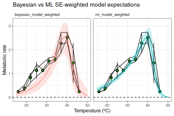
Let’s compare the models
1
2
3
4
5
6
7
8
9
10
11
12
13
14
15
16
17
18
19
20
21
22
23
24
25
26
27
28
29
30
31
32
33
34
35
36
37
38
39
40
41
42
43
44
45
46
47
48
49
50
51
52
53
54
55
56
57
58
59
60
61
| nd <- data.frame(
temp=seq(15,50,by=0.1)
)
nd %>%
predictions(
ml_model_weighted,
newdata = .,
type = "fitted"
) %>%
select(temp, estimate, conf.low, conf.high) %>%
mutate(model = "ml_model_weighted") %>%
bind_rows(
bind_cols(
nd,
fitted(
bayesian_model_weighted,
# se column needs to be in the model, but is ignored when getting fitted values
# (changing it does not affect the plots)
newdata = nd %>% mutate(se = mean(d_ave$se)),
allow_new_levels = TRUE
)
) %>%
as.data.frame() %>%
select(temp, estimate = Estimate, conf.low = Q2.5, conf.high = Q97.5) %>%
mutate(model = "bayesian_model_weighted")
) %>%
as_tibble() %>%
ggplot(aes(x = temp, y = estimate)) +
theme_bw(base_size = 12) +
theme(legend.position = 'none',
strip.text = element_text(hjust = 0),
strip.background = element_blank()) +
labs(x ='Temperature (ºC)',
y = 'Metabolic rate',
title = 'Bayesian vs ML SE-weighted model expectations') +
geom_hline(aes(yintercept = 0), linetype = 2) +
# add the observed data
geom_line(
aes(y = rate, group = curve_id),
data = filter(
chlorella_tpc,
process == 'adaptation',
growth_temp == 33,
flux == 'photosynthesis'
) %>%
mutate(curve_id = as.factor(curve_id)) %>%
as_tibble()
) +
geom_pointrange(
aes(y = ave_rate, ymax = ave_rate + sd, ymin = ave_rate - sd),
shape = 21, fill = 'green4',
data = d_ave
) +
geom_line(aes(colour = model),show.legend = F) +
geom_ribbon(
aes(fill = model, ymin = conf.low, ymax = conf.high),
alpha = 0.2,
show.legend = F
) +
facet_wrap(~model, nrow = 1)
|
1
2
3
4
5
6
7
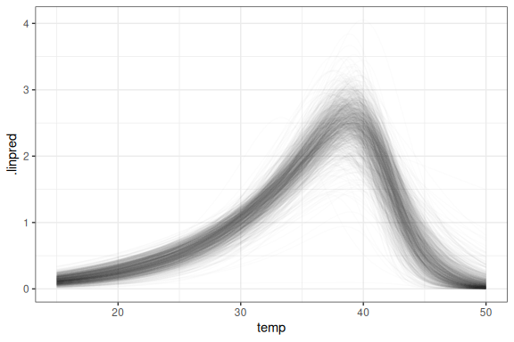
| # We can also look at the posterior draws to see where the Bayesian model's uncertainty comes from
nd %>%
mutate(se=1) %>% # ignored
add_linpred_draws(bayesian_model_weighted,ndraws=1000) %>%
ggplot(aes(x=temp,y=.linpred))+
geom_line(aes(group=.draw),alpha=.01)
|
Hierarchical method
Now, it turns out that fitting the Pawar (2018) model to this data in a fully hierarchical manner is quite difficult, but there is a neat alternative which I’ll describe later. But for now, let’s give it a go.
1
2
3
4
5
6
7
8
9
10
| # Don't do any averaging!
d_hier <- filter(
chlorella_tpc,
process == 'adaptation',
growth_temp == 33,
flux == 'photosynthesis'
) %>%
mutate(curve_id = as.factor(curve_id)) %>%
as_tibble()
d_hier
|
1
2
3
4
5
6
7
8
9
10
11
12
13
14
| ## # A tibble: 30 × 6
## curve_id growth_temp process flux temp rate
## <fct> <dbl> <chr> <chr> <dbl> <dbl>
## 1 58 33 adaptation photosynthesis 16 0.221
## 2 58 33 adaptation photosynthesis 19 0.300
## 3 58 33 adaptation photosynthesis 22 0.622
## 4 58 33 adaptation photosynthesis 25 0.876
## 5 58 33 adaptation photosynthesis 28 1.09
## 6 58 33 adaptation photosynthesis 31 1.40
## 7 58 33 adaptation photosynthesis 34 1.50
## 8 58 33 adaptation photosynthesis 37 1.89
## 9 58 33 adaptation photosynthesis 40 2.50
## 10 58 33 adaptation photosynthesis 43 0.851
## # ℹ 20 more rows
|
1
2
3
4
5
6
7
8
9
10
11
12
13
14
15
16
17
18
19
20
21
22
23
24
25
26
27
28
29
30
31
32
| # Start with just random effects on t_opt
bform_hier_topt <- bf(
rate ~ pawar_2018a(temp, rtref, e, eh, topt),
rtref ~ 1 ,
e ~ 1,
eh ~ 1 ,
topt ~ 1 + (1 | curve_id), # <---- Note the familiar syntax used here :)
nl = TRUE
)
# Update the priors
priors_hier <- c(
priors,
# half-normal with low sd -- close to zero
prior(normal(0,0.3),lb=0,class="sd",nlpar="topt")
)
bayesian_model_hier_topt <- brm(
bform_hier_topt,
family = brmsfamily("gaussian"),
data = d_hier,
stanvars = stanvars_pawar_2018a,
prior = priors_hier,
control = list(adapt_delta = 0.999, max_treedepth = 15),
cores = 4,
iter = 4000,
warmup = 3000,
refresh = 1000,
backend = "cmdstanr",
file = ".brms/pawar-h1"
)
summary(bayesian_model_hier_topt)
|
1
2
3
4
5
6
7
8
9
10
11
12
13
14
15
16
17
18
19
20
21
22
23
24
25
26
27
28
29
30
| ## Family: gaussian
## Links: mu = identity
## Formula: rate ~ pawar_2018a(temp, rtref, e, eh, topt)
## rtref ~ 1
## e ~ 1
## eh ~ 1
## topt ~ 1 + (1 | curve_id)
## Data: d_hier (Number of observations: 30)
## Draws: 4 chains, each with iter = 4000; warmup = 3000; thin = 1;
## total post-warmup draws = 4000
##
## Multilevel Hyperparameters:
## ~curve_id (Number of levels: 3)
## Estimate Est.Error l-95% CI u-95% CI Rhat Bulk_ESS Tail_ESS
## sd(topt_Intercept) 0.37 0.20 0.02 0.79 1.00 974 834
##
## Regression Coefficients:
## Estimate Est.Error l-95% CI u-95% CI Rhat Bulk_ESS Tail_ESS
## rtref_Intercept 0.40 0.06 0.27 0.52 1.00 1470 1820
## e_Intercept 0.83 0.09 0.68 1.05 1.00 1365 1727
## eh_Intercept 6.23 1.03 4.39 8.43 1.00 1615 2187
## topt_Intercept 39.25 0.46 38.25 39.95 1.00 1499 1211
##
## Further Distributional Parameters:
## Estimate Est.Error l-95% CI u-95% CI Rhat Bulk_ESS Tail_ESS
## sigma 0.29 0.06 0.20 0.41 1.00 1223 2347
##
## Draws were sampled using sample(hmc). For each parameter, Bulk_ESS
## and Tail_ESS are effective sample size measures, and Rhat is the potential
## scale reduction factor on split chains (at convergence, Rhat = 1).
|
1
2
3
4
5
6
7
8
9
10
11
12
13
14
15
16
17
18
19
20
21
22
23
24
25
26
27
28
29
30
31
32
33
| # Add a random effect on eh? (deactivation energy might vary among individuals)
bform_hier_topt_eh <- bf(
rate ~ pawar_2018a(temp, rtref, e, eh, topt),
rtref ~ 1 ,
e ~ 1,
eh ~ 1 + (1 | curve_id),
topt ~ 1 + (1 | curve_id),
nl = TRUE
)
# Update the priors
priors_hier <- c(
priors,
# half-normal with low sd -- close to zero
prior(normal(0,0.3),lb=0,class="sd",nlpar="topt"),
prior(normal(0,0.3),lb=0,class="sd",nlpar="eh")
)
bayesian_model_hier_topt_eh <- brm(
bform_hier_topt_eh,
family = brmsfamily("gaussian"),
data = d_hier,
stanvars = stanvars_pawar_2018a,
prior = priors_hier,
control = list(adapt_delta = 0.999, max_treedepth = 15),
cores = 4,
iter = 4000,
warmup = 3000,
refresh = 1000,
backend = "cmdstanr",
file = ".brms/pawar-h2"
)
summary(bayesian_model_hier_topt_eh)
|
1
2
3
4
5
6
7
8
9
10
11
12
13
14
15
16
17
18
19
20
21
22
23
24
25
26
27
28
29
30
31
32
33
34
35
36
37
38
39
| ## Warning: Parts of the model have not converged (some Rhats are > 1.05). Be
## careful when analysing the results! We recommend running more iterations and/or
## setting stronger priors.
## Warning: There were 955 divergent transitions after warmup. Increasing
## adapt_delta above 0.999 may help. See
## http://mc-stan.org/misc/warnings.html#divergent-transitions-after-warmup
## Family: gaussian
## Links: mu = identity
## Formula: rate ~ pawar_2018a(temp, rtref, e, eh, topt)
## rtref ~ 1
## e ~ 1
## eh ~ 1 + (1 | curve_id)
## topt ~ 1 + (1 | curve_id)
## Data: d_hier (Number of observations: 30)
## Draws: 4 chains, each with iter = 4000; warmup = 3000; thin = 1;
## total post-warmup draws = 4000
##
## Multilevel Hyperparameters:
## ~curve_id (Number of levels: 3)
## Estimate Est.Error l-95% CI u-95% CI Rhat Bulk_ESS Tail_ESS
## sd(eh_Intercept) 0.42 0.36 0.01 1.18 1.52 7 32
## sd(topt_Intercept) 0.35 0.21 0.02 0.79 1.02 301 662
##
## Regression Coefficients:
## Estimate Est.Error l-95% CI u-95% CI Rhat Bulk_ESS Tail_ESS
## rtref_Intercept 0.30 0.18 0.00 0.51 1.54 7 25
## e_Intercept 1.02 0.33 0.69 1.82 1.53 7 33
## eh_Intercept 5.04 2.12 1.41 8.15 1.53 7 24
## topt_Intercept 39.33 0.46 38.23 39.97 1.11 25 169
##
## Further Distributional Parameters:
## Estimate Est.Error l-95% CI u-95% CI Rhat Bulk_ESS Tail_ESS
## sigma 0.57 0.50 0.21 1.68 1.53 7 36
##
## Draws were sampled using sample(hmc). For each parameter, Bulk_ESS
## and Tail_ESS are effective sample size measures, and Rhat is the potential
## scale reduction factor on split chains (at convergence, Rhat = 1).
|
1
2
3
4
5
6
7
8
9
10
11
12
13
14
15
16
17
18
19
20
21
| nd %>%
add_linpred_draws(bayesian_model_hier_topt_eh,ndraws=1000,re_formula = NA) %>%
ggplot(aes(x=temp,y=.linpred))+
geom_line(aes(group=.draw),alpha=.01)+
# add the observed data
geom_line(
aes(y = rate, group = curve_id),
data = filter(
chlorella_tpc,
process == 'adaptation',
growth_temp == 33,
flux == 'photosynthesis'
) %>%
mutate(curve_id = as.factor(curve_id)) %>%
as_tibble()
) +
geom_pointrange(
aes(y = ave_rate, ymax = ave_rate + sd, ymin = ave_rate - sd),
shape = 21, fill = 'green4',
data = d_ave
)
|
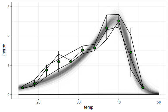
Allowing $t_{opt}$ to vary among individuals worked fine, but for $eh$… eh. Not so good. This is probably overkil, as we only have 3 colonies! But what if we wanted to test whether the curves differed between colonies grown at different temperatures? Now we can use the full power of this approach.
Getting really fancy: The one TPC to rule them all!
Before doing so, I’ll switch over to using a different model which is hot off the press and quite spectacular. It’s billed as a “universal thermal performance curve” by the Arnoldi et al. (2025) and has a remarkably simple formulation, with three parameters representing the optimal temperature $T_{opt}$, the rate at that optimum $y_{opt}$, and the difference between $T_{opt}$ and the critical upper limit $Delta$. Temperature is in Celcius (I know, crazy!).
\[\mathrm{rate} = y_{\mathrm{opt}}\times \exp\!\left(\frac{T - T_{\mathrm{opt}}}{\Delta}\right)\times \left(1 - \frac{T - T_{\mathrm{opt}}}{\Delta}\right)\]
Fit the universal TPC
The simplicity of the formula means we can write much more concise code.
1
2
3
4
5
6
7
8
9
10
11
12
13
14
15
16
17
18
19
20
21
22
23
24
25
26
27
28
29
30
31
32
33
34
35
36
37
38
39
| # Model -------------------------------------------------------------------
# See https://github.com/AndrewLJackson/UTPC-paper/blob/main/import-fit-merge.Rmd#L132C9-L132C68
# performance ~ (yopt * exp( (ta - Topt)/Delta ) * (1 - (ta - Topt)/Delta))
# ta = temp in Celcius!
bform <- bf(
rate ~ yopt * exp((temp - Topt) / Delta) * (1 - (temp - Topt) / Delta),
yopt ~ 1 + (1 | curve_id),
Topt ~ 1 + (1 | curve_id),
Delta ~ 1 + (1 | curve_id),
nl = TRUE
)
priors <- c(
prior(normal(2, 0.25), lb = 0, nlpar = "yopt"),
prior(normal(1, 3), lb = 0, ub = 20, nlpar = "Delta"),
prior(normal(40, 3), lb = 30, ub = 50, nlpar = "Topt"),
prior(normal(0, 0.3), lb = 0, class = "sd", nlpar = "yopt"),
prior(std_normal(), lb = 0, class = "sd", nlpar = "Topt"),
prior(normal(0, 0.3), lb = 0, class = "sd", nlpar = "Delta"),
prior(normal(0, 0.1), lb = 0, class = "sigma")
)
m_UTPC <- brm(
bform,
family = brmsfamily("gaussian"),
data = d_hier,
prior = priors,
control = list(adapt_delta = 0.99, max_treedepth = 12),
cores = 4,
iter = 2000,
warmup = 1500,
refresh = 500,
backend = "cmdstanr",
file = ".brms/utpc-1"
)
m_UTPC
|
1
2
3
4
5
6
7
8
9
10
11
12
13
14
15
16
17
18
19
20
21
22
23
24
25
26
27
28
29
30
| ## Family: gaussian
## Links: mu = identity
## Formula: rate ~ yopt * exp((temp - Topt)/Delta) * (1 - (temp - Topt)/Delta)
## yopt ~ 1 + (1 | curve_id)
## Topt ~ 1 + (1 | curve_id)
## Delta ~ 1 + (1 | curve_id)
## Data: d_hier (Number of observations: 30)
## Draws: 4 chains, each with iter = 2000; warmup = 1500; thin = 1;
## total post-warmup draws = 2000
##
## Multilevel Hyperparameters:
## ~curve_id (Number of levels: 3)
## Estimate Est.Error l-95% CI u-95% CI Rhat Bulk_ESS Tail_ESS
## sd(yopt_Intercept) 0.29 0.14 0.08 0.61 1.00 576 311
## sd(Topt_Intercept) 0.35 0.33 0.01 1.29 1.00 937 1258
## sd(Delta_Intercept) 0.18 0.15 0.01 0.55 1.00 1167 768
##
## Regression Coefficients:
## Estimate Est.Error l-95% CI u-95% CI Rhat Bulk_ESS Tail_ESS
## yopt_Intercept 2.17 0.15 1.86 2.45 1.00 1127 1218
## Topt_Intercept 39.19 0.38 38.41 39.93 1.01 892 1116
## Delta_Intercept 7.07 0.33 6.39 7.73 1.00 1232 1381
##
## Further Distributional Parameters:
## Estimate Est.Error l-95% CI u-95% CI Rhat Bulk_ESS Tail_ESS
## sigma 0.24 0.03 0.19 0.30 1.00 1728 1544
##
## Draws were sampled using sample(hmc). For each parameter, Bulk_ESS
## and Tail_ESS are effective sample size measures, and Rhat is the potential
## scale reduction factor on split chains (at convergence, Rhat = 1).
|
1
2
3
4
| plot(
conditional_effects(m_UTPC, effects = "temp", spaghetti = T, ndraws = 500),
points = T
)
|
1
2
3
4
| ## Ignoring unknown labels:
## • colour : "NA"
## Ignoring unknown labels:
## • colour : "NA"
|
1
2
3
4
5
6
7
8
9
10
11
12
13
14
15
| nd %>%
add_linpred_draws(m_UTPC,ndraws=1000,re_formula = NA) %>%
ggplot(aes(x=temp,y=.linpred))+
geom_line(aes(group=.draw),alpha=.01)+
# add the observed data
geom_line(
aes(y = rate, group = curve_id),
data = d_hier
) +
geom_pointrange(
aes(y = ave_rate, ymax = ave_rate + sd, ymin = ave_rate - sd),
shape = 21, fill = 'green4',
data = d_ave
) +
coord_cartesian(ylim=c(0,3))
|
1
| pp_check(m_UTPC, ndraws = 100)
|
1
2
| # Compare to the pawar model that converged
loo(bayesian_model_hier_topt,m_UTPC)
|
1
2
3
4
5
6
7
8
9
10
11
12
13
14
15
16
17
18
19
20
21
22
23
24
25
26
27
28
29
30
31
32
33
34
35
36
37
38
39
40
41
42
43
44
45
46
47
48
49
50
| ## Warning: Found 1 observations with a pareto_k > 0.7 in model
## 'bayesian_model_hier_topt'. We recommend to set 'moment_match = TRUE' in order
## to perform moment matching for problematic observations.
## Warning: Found 4 observations with a pareto_k > 0.7 in model 'm_UTPC'. We
## recommend to set 'moment_match = TRUE' in order to perform moment matching for
## problematic observations.
## Output of model 'bayesian_model_hier_topt':
##
## Computed from 4000 by 30 log-likelihood matrix.
##
## Estimate SE
## elpd_loo -8.7 4.6
## p_loo 6.3 2.2
## looic 17.4 9.2
## ------
## MCSE of elpd_loo is NA.
## MCSE and ESS estimates assume MCMC draws (r_eff in [0.3, 0.9]).
##
## Pareto k diagnostic values:
## Count Pct. Min. ESS
## (-Inf, 0.7] (good) 29 96.7% 293
## (0.7, 1] (bad) 1 3.3% <NA>
## (1, Inf) (very bad) 0 0.0% <NA>
## See help('pareto-k-diagnostic') for details.
##
## Output of model 'm_UTPC':
##
## Computed from 2000 by 30 log-likelihood matrix.
##
## Estimate SE
## elpd_loo -9.2 7.7
## p_loo 10.1 3.8
## looic 18.4 15.3
## ------
## MCSE of elpd_loo is NA.
## MCSE and ESS estimates assume MCMC draws (r_eff in [0.4, 1.5]).
##
## Pareto k diagnostic values:
## Count Pct. Min. ESS
## (-Inf, 0.7] (good) 26 86.7% 358
## (0.7, 1] (bad) 2 6.7% <NA>
## (1, Inf) (very bad) 2 6.7% <NA>
## See help('pareto-k-diagnostic') for details.
##
## Model comparisons:
## elpd_diff se_diff
## bayesian_model_hier_topt 0.0 0.0
## m_UTPC -0.5 7.8
|
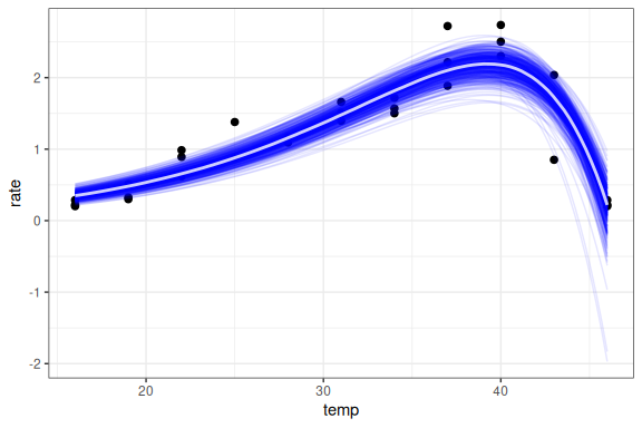
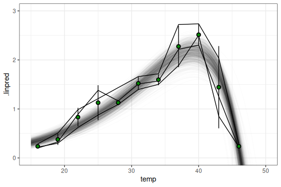
The model has no problem fitting random effects on every parameter, despite only having three replicates. Notice also that the model is not constrained to rates above 0 beyond $T_{opt}$. This is because it assumes a function that crosses zero at the critical temperature, i.e., we expect anything beyond that point to be dead…
Test some hypotheses!
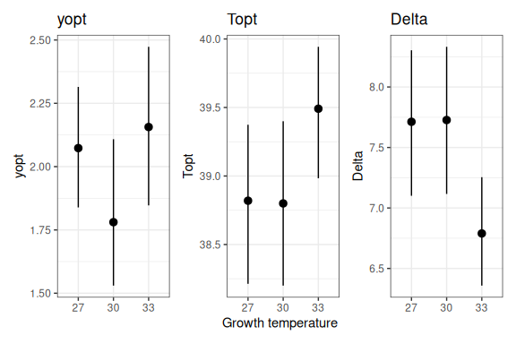
Heartened by how easily the UTPC model fit, we could try testing some biological hypotheses. Arnoldi et al. suggested that, under a warming scenario, the upper thermal limit is a much “harder” trait for natural selection to act on compared to the thermal optimum. As such, we would expect our algae grown at higher temperatures to have higher $T_{opt}$ and lower $Delta$, i.e., a steeper drop-off and a narrower range of good performance.
Let’s test that prediction by allowing our parameters to vary by growth temperature. We also estimate separate random effect SDs for each growth temperature.
1
2
3
4
5
6
7
8
9
10
11
12
13
14
15
16
17
18
19
20
21
22
23
24
25
26
27
28
29
30
31
32
33
34
35
| d_hier_3temp <- filter(
chlorella_tpc,
process == 'adaptation',
growth_temp %in% c(27, 30, 33),
flux == 'photosynthesis'
) %>%
mutate(
curve_id = as.factor(curve_id),
growth_temp_fct = as.factor(growth_temp)
)
bform_UTPC_3temp <- bf(
rate ~ yopt * exp((temp - Topt) / Delta) * (1 - (temp - Topt) / Delta),
yopt ~ 0 + (1 | gr(curve_id,by=growth_temp_fct)) + growth_temp_fct,
Topt ~ 0 + (1 | gr(curve_id,by=growth_temp_fct)) + growth_temp_fct,
Delta ~ 0 + (1 | gr(curve_id,by=growth_temp_fct)) + growth_temp_fct,
nl = TRUE
)
m_UTPC_3temp <- brm(
bform_UTPC_3temp,
family = brmsfamily("gaussian"),
data = d_hier_3temp,
prior = priors,
# sample_prior = "only",
control = list(adapt_delta = 0.99, max_treedepth = 12),
cores = 4,
iter = 2000,
warmup = 1500,
refresh = 500,
backend = "cmdstanr",
file = ".brms/utpc-2",
seed = 1234
)
m_UTPC_3temp
|
1
2
3
4
5
6
7
8
9
10
11
12
13
14
15
16
17
18
19
20
21
22
23
24
25
26
27
28
29
30
31
32
33
34
35
36
37
38
39
40
41
42
43
44
45
46
47
48
49
50
51
52
53
54
55
56
57
58
59
60
61
62
| ## Family: gaussian
## Links: mu = identity
## Formula: rate ~ yopt * exp((temp - Topt)/Delta) * (1 - (temp - Topt)/Delta)
## yopt ~ 0 + (1 | gr(curve_id, by = growth_temp_fct)) + growth_temp_fct
## Topt ~ 0 + (1 | gr(curve_id, by = growth_temp_fct)) + growth_temp_fct
## Delta ~ 0 + (1 | gr(curve_id, by = growth_temp_fct)) + growth_temp_fct
## Data: d_hier_3temp (Number of observations: 96)
## Draws: 4 chains, each with iter = 2000; warmup = 1500; thin = 1;
## total post-warmup draws = 2000
##
## Multilevel Hyperparameters:
## ~curve_id (Number of levels: 9)
## Estimate Est.Error l-95% CI u-95% CI Rhat
## sd(yopt_Intercept:growth_temp_fct27) 0.10 0.10 0.00 0.36 1.00
## sd(yopt_Intercept:growth_temp_fct30) 0.22 0.13 0.03 0.52 1.00
## sd(yopt_Intercept:growth_temp_fct33) 0.31 0.13 0.11 0.62 1.00
## sd(Topt_Intercept:growth_temp_fct27) 0.35 0.35 0.01 1.33 1.01
## sd(Topt_Intercept:growth_temp_fct30) 0.38 0.37 0.01 1.38 1.00
## sd(Topt_Intercept:growth_temp_fct33) 0.33 0.33 0.01 1.23 1.01
## sd(Delta_Intercept:growth_temp_fct27) 0.18 0.15 0.01 0.55 1.00
## sd(Delta_Intercept:growth_temp_fct30) 0.20 0.16 0.01 0.59 1.00
## sd(Delta_Intercept:growth_temp_fct33) 0.17 0.14 0.01 0.52 1.00
## Bulk_ESS Tail_ESS
## sd(yopt_Intercept:growth_temp_fct27) 872 1092
## sd(yopt_Intercept:growth_temp_fct30) 744 595
## sd(yopt_Intercept:growth_temp_fct33) 1358 1314
## sd(Topt_Intercept:growth_temp_fct27) 898 1056
## sd(Topt_Intercept:growth_temp_fct30) 903 905
## sd(Topt_Intercept:growth_temp_fct33) 885 806
## sd(Delta_Intercept:growth_temp_fct27) 1457 992
## sd(Delta_Intercept:growth_temp_fct30) 1326 1036
## sd(Delta_Intercept:growth_temp_fct33) 1648 1118
##
## Regression Coefficients:
## Estimate Est.Error l-95% CI u-95% CI Rhat Bulk_ESS
## yopt_growth_temp_fct27 2.09 0.09 1.89 2.26 1.00 1310
## yopt_growth_temp_fct30 1.80 0.13 1.55 2.08 1.00 1256
## yopt_growth_temp_fct33 2.16 0.16 1.84 2.46 1.00 1127
## Topt_growth_temp_fct27 38.66 0.41 37.81 39.43 1.00 1545
## Topt_growth_temp_fct30 38.90 0.44 38.05 39.79 1.00 1272
## Topt_growth_temp_fct33 39.18 0.35 38.43 39.87 1.00 1451
## Delta_growth_temp_fct27 7.79 0.33 7.18 8.46 1.00 1901
## Delta_growth_temp_fct30 7.62 0.39 6.88 8.44 1.00 2052
## Delta_growth_temp_fct33 7.07 0.28 6.54 7.63 1.00 2170
## Tail_ESS
## yopt_growth_temp_fct27 719
## yopt_growth_temp_fct30 1370
## yopt_growth_temp_fct33 1141
## Topt_growth_temp_fct27 1126
## Topt_growth_temp_fct30 1056
## Topt_growth_temp_fct33 1137
## Delta_growth_temp_fct27 1487
## Delta_growth_temp_fct30 1411
## Delta_growth_temp_fct33 1413
##
## Further Distributional Parameters:
## Estimate Est.Error l-95% CI u-95% CI Rhat Bulk_ESS Tail_ESS
## sigma 0.21 0.02 0.18 0.25 1.00 2229 1235
##
## Draws were sampled using sample(hmc). For each parameter, Bulk_ESS
## and Tail_ESS are effective sample size measures, and Rhat is the potential
## scale reduction factor on split chains (at convergence, Rhat = 1).
|
Reparameterise as log-normal
This model sometimes has trouble sampling, depending on the random seed, so I tried reformulating it in logarithmic form. The formula then becomes:
\[log\mathrm{(rate)} = log(y_{\mathrm{opt}}) + \left(\frac{T - T_{\mathrm{opt}}}{\Delta}\right) + log\left(1 - \frac{T - T_{\mathrm{opt}}}{\Delta}\right)\]
And we just need to change the family to lognormal. Everything else remains unchanged, even the priors!
1
2
3
4
5
6
7
8
9
10
11
12
13
14
15
16
17
18
19
20
21
22
23
| bform_UTPC_3temp_lognormal <- bf(
rate ~ log(yopt) + ((temp - Topt) / Delta) + log(1 - (temp - Topt) / Delta),
yopt ~ 0 + (1 | gr(curve_id,by=growth_temp_fct)) + growth_temp_fct,
Topt ~ 0 + (1 | gr(curve_id,by=growth_temp_fct)) + growth_temp_fct,
Delta ~ 0 + (1 | gr(curve_id,by=growth_temp_fct)) + growth_temp_fct,
nl = TRUE
)
m_UTPC_3temp_lognormal <- brm(
bform_UTPC_3temp_lognormal,
family = brmsfamily("lognormal"),
data = d_hier_3temp,
prior = priors,
control = list(adapt_delta = 0.99, max_treedepth = 12),
cores = 4,
iter = 2000,
warmup = 1500,
refresh = 500,
backend = "cmdstanr",
file = ".brms/utpc-2-log",
seed = 123
)
m_UTPC_3temp_lognormal
|
1
2
3
4
5
6
7
8
9
10
11
12
13
14
15
16
17
18
19
20
21
22
23
24
25
26
27
28
29
30
31
32
33
34
35
36
37
38
39
40
41
42
43
44
45
46
47
48
49
50
51
52
53
54
55
56
57
58
59
60
61
62
63
64
65
66
| ## Warning: There were 1 divergent transitions after warmup. Increasing
## adapt_delta above 0.99 may help. See
## http://mc-stan.org/misc/warnings.html#divergent-transitions-after-warmup
## Family: lognormal
## Links: mu = identity
## Formula: rate ~ log(yopt) + ((temp - Topt)/Delta) + log(1 - (temp - Topt)/Delta)
## yopt ~ 0 + (1 | gr(curve_id, by = growth_temp_fct)) + growth_temp_fct
## Topt ~ 0 + (1 | gr(curve_id, by = growth_temp_fct)) + growth_temp_fct
## Delta ~ 0 + (1 | gr(curve_id, by = growth_temp_fct)) + growth_temp_fct
## Data: d_hier_3temp (Number of observations: 96)
## Draws: 4 chains, each with iter = 2000; warmup = 1500; thin = 1;
## total post-warmup draws = 2000
##
## Multilevel Hyperparameters:
## ~curve_id (Number of levels: 9)
## Estimate Est.Error l-95% CI u-95% CI Rhat
## sd(yopt_Intercept:growth_temp_fct27) 0.12 0.10 0.01 0.38 1.00
## sd(yopt_Intercept:growth_temp_fct30) 0.24 0.13 0.04 0.56 1.00
## sd(yopt_Intercept:growth_temp_fct33) 0.28 0.15 0.04 0.62 1.00
## sd(Topt_Intercept:growth_temp_fct27) 0.23 0.27 0.01 1.03 1.00
## sd(Topt_Intercept:growth_temp_fct30) 0.27 0.30 0.01 1.10 1.01
## sd(Topt_Intercept:growth_temp_fct33) 0.18 0.24 0.00 0.86 1.00
## sd(Delta_Intercept:growth_temp_fct27) 0.15 0.13 0.01 0.48 1.00
## sd(Delta_Intercept:growth_temp_fct30) 0.20 0.15 0.01 0.58 1.00
## sd(Delta_Intercept:growth_temp_fct33) 0.13 0.12 0.00 0.45 1.00
## Bulk_ESS Tail_ESS
## sd(yopt_Intercept:growth_temp_fct27) 1320 1255
## sd(yopt_Intercept:growth_temp_fct30) 916 819
## sd(yopt_Intercept:growth_temp_fct33) 890 590
## sd(Topt_Intercept:growth_temp_fct27) 992 1119
## sd(Topt_Intercept:growth_temp_fct30) 682 837
## sd(Topt_Intercept:growth_temp_fct33) 748 1059
## sd(Delta_Intercept:growth_temp_fct27) 1079 1104
## sd(Delta_Intercept:growth_temp_fct30) 886 691
## sd(Delta_Intercept:growth_temp_fct33) 941 1062
##
## Regression Coefficients:
## Estimate Est.Error l-95% CI u-95% CI Rhat Bulk_ESS
## yopt_growth_temp_fct27 2.07 0.12 1.84 2.31 1.00 1773
## yopt_growth_temp_fct30 1.79 0.15 1.53 2.11 1.00 1442
## yopt_growth_temp_fct33 2.16 0.16 1.85 2.47 1.00 1530
## Topt_growth_temp_fct27 38.81 0.29 38.21 39.37 1.00 1418
## Topt_growth_temp_fct30 38.80 0.31 38.20 39.40 1.00 1273
## Topt_growth_temp_fct33 39.48 0.25 38.98 39.94 1.00 1005
## Delta_growth_temp_fct27 7.71 0.30 7.10 8.30 1.00 1472
## Delta_growth_temp_fct30 7.72 0.31 7.12 8.33 1.00 1445
## Delta_growth_temp_fct33 6.80 0.23 6.36 7.25 1.00 1306
## Tail_ESS
## yopt_growth_temp_fct27 1370
## yopt_growth_temp_fct30 1353
## yopt_growth_temp_fct33 1452
## Topt_growth_temp_fct27 1306
## Topt_growth_temp_fct30 921
## Topt_growth_temp_fct33 841
## Delta_growth_temp_fct27 1329
## Delta_growth_temp_fct30 1125
## Delta_growth_temp_fct33 1287
##
## Further Distributional Parameters:
## Estimate Est.Error l-95% CI u-95% CI Rhat Bulk_ESS Tail_ESS
## sigma 0.21 0.02 0.18 0.24 1.00 1961 1459
##
## Draws were sampled using sample(hmc). For each parameter, Bulk_ESS
## and Tail_ESS are effective sample size measures, and Rhat is the potential
## scale reduction factor on split chains (at convergence, Rhat = 1).
|
I think this works because working in log space is more numerically stable, but I’m not really sure. Anyway, it works!
Was our prediction correct?
1
2
3
4
5
6
7
8
9
10
11
12
13
14
15
16
17
18
19
20
21
22
23
| yopt_plot <- plot_predictions(
m_UTPC_3temp_lognormal,
condition = c("growth_temp_fct"),
nlpar="yopt",
points = .5,
re_formula = NA
)+labs(y="yopt",title="yopt",x="Growth temperature")
Topt_plot <- plot_predictions(
m_UTPC_3temp_lognormal,
condition = c("growth_temp_fct"),
nlpar="Topt",
points = .5,
re_formula = NA
)+labs(y="Topt",title="Topt",x="Growth temperature")
Delta_plot <- plot_predictions(
m_UTPC_3temp_lognormal,
condition = c("growth_temp_fct"),
nlpar="Delta",
points = .5,
re_formula = NA
)+labs(y="Delta",title="Delta",x="Growth temperature")
patchwork::wrap_plots(yopt_plot,Topt_plot,Delta_plot,axes = "collect")
|
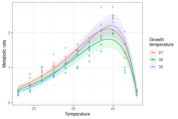
Remarkably, the prediction seems to be right. The colonies grown at 33 degrees for ~ 100 generations had a higher thermal optimum (by around 0.7 ${^\circ}C$) but lower $Delta$ (by around 0.9 ${^\circ}C$) than those grown at lower temperatures, implying that the upper thermal limit didn’t change, or may have even declined…
Finally, let’s look at some predictions.
1
2
3
4
5
6
7
8
| plot_predictions(
m_UTPC_3temp_lognormal,
condition = c("temp", "growth_temp_fct"),
points = .5,
re_formula = NA
)+
labs(fill="Growth\ntemperature",colour="Growth\ntemperature",
x="Temperature",y="Metabolic rate")
|
References
Kontopoulos, D..G., Sentis, A., Daufresne, M. et al. (2024) No universal mathematical model for thermal performance curves across traits and taxonomic groups. Nat Commun 15, 8855. https://doi.org/10.1038/s41467-024-53046-2
Padfield, D., Yvon-durocher, G., Buckling, A., Jennings, S. & Yvon-durocher, G. (2015). Rapid evolution of metabolic traits explains thermal adaptation in phytoplankton, Ecology Letters, 19, 133-142.
J. Arnoldi, A.L. Jackson, I. Peralta-Maraver, & N.L. Payne. (2025) A universal thermal performance curve arises in biology and ecology, Proc. Natl. Acad. Sci. U.S.A. 122 (43) e2513099122, https://doi.org/10.1073/pnas.2513099122.
1
2
3
4
5
6
7
8
9
10
11
12
13
14
15
16
17
18
19
20
21
22
23
24
25
26
27
28
29
30
31
32
33
34
35
36
37
38
39
40
41
42
43
44
45
46
47
48
49
50
51
52
53
54
55
56
57
58
59
| ## R version 4.5.2 (2025-10-31)
## Platform: x86_64-pc-linux-gnu
## Running under: Linux Mint 22.1
##
## Matrix products: default
## BLAS: /usr/lib/x86_64-linux-gnu/blas/libblas.so.3.12.0
## LAPACK: /usr/lib/x86_64-linux-gnu/lapack/liblapack.so.3.12.0 LAPACK version 3.12.0
##
## locale:
## [1] LC_CTYPE=en_ZA.UTF-8 LC_NUMERIC=C
## [3] LC_TIME=en_ZA.UTF-8 LC_COLLATE=en_ZA.UTF-8
## [5] LC_MONETARY=en_ZA.UTF-8 LC_MESSAGES=en_ZA.UTF-8
## [7] LC_PAPER=en_ZA.UTF-8 LC_NAME=C
## [9] LC_ADDRESS=C LC_TELEPHONE=C
## [11] LC_MEASUREMENT=en_ZA.UTF-8 LC_IDENTIFICATION=C
##
## time zone: Africa/Johannesburg
## tzcode source: system (glibc)
##
## attached base packages:
## [1] stats graphics grDevices datasets utils methods base
##
## other attached packages:
## [1] tidybayes_3.0.7 ggdist_3.3.3 marginaleffects_0.31.0
## [4] brms_2.23.0 Rcpp_1.1.0 ggrepel_0.9.6
## [7] lubridate_1.9.4 forcats_1.0.1 stringr_1.6.0
## [10] dplyr_1.1.4 purrr_1.2.0 readr_2.1.6
## [13] tidyr_1.3.1 tibble_3.3.0 ggplot2_4.0.1
## [16] tidyverse_2.0.0 rTPC_1.0.4 knitr_1.50
##
## loaded via a namespace (and not attached):
## [1] tidyselect_1.2.1 svUnit_1.0.8 farver_2.1.2
## [4] loo_2.8.0 S7_0.2.1 fastmap_1.2.0
## [7] tensorA_0.36.2.1 digest_0.6.39 estimability_1.5.1
## [10] timechange_0.3.0 lifecycle_1.0.4 StanHeaders_2.32.10
## [13] processx_3.8.6 magrittr_2.0.4 posterior_1.6.1
## [16] compiler_4.5.2 rlang_1.1.6 tools_4.5.2
## [19] utf8_1.2.6 yaml_2.3.10 collapse_2.1.5
## [22] data.table_1.17.8 labeling_0.4.3 bridgesampling_1.2-1
## [25] curl_7.0.0 pkgbuild_1.4.8 plyr_1.8.9
## [28] RColorBrewer_1.1-3 cmdstanr_0.9.0 abind_1.4-8
## [31] withr_3.0.2 grid_4.5.2 stats4_4.5.2
## [34] colorspace_2.1-2 xtable_1.8-4 inline_0.3.21
## [37] emmeans_2.0.0 scales_1.4.0 insight_1.4.2
## [40] dichromat_2.0-0.1 cli_3.6.5 mvtnorm_1.3-3
## [43] rmarkdown_2.30 generics_0.1.4 RcppParallel_5.1.11-1
## [46] rstudioapi_0.17.1 reshape2_1.4.5 tzdb_0.5.0
## [49] rstan_2.32.7 bayesplot_1.14.0 parallel_4.5.2
## [52] matrixStats_1.5.0 vctrs_0.6.5 V8_8.0.1
## [55] Matrix_1.7-4 jsonlite_2.0.0 minpack.lm_1.2-4
## [58] patchwork_1.3.2 hms_1.1.4 arrayhelpers_1.1-0
## [61] glue_1.8.0 codetools_0.2-20 ps_1.9.1
## [64] distributional_0.5.0 stringi_1.8.7 gtable_0.3.6
## [67] QuickJSR_1.8.1 bspm_0.5.7 pillar_1.11.1
## [70] htmltools_0.5.8.1 Brobdingnag_1.2-9 R6_2.6.1
## [73] evaluate_1.0.5 lattice_0.22-7 backports_1.5.0
## [76] nls.multstart_2.0.0 rstantools_2.5.0 coda_0.19-4.1
## [79] gridExtra_2.3 nlme_3.1-168 checkmate_2.3.3
## [82] xfun_0.54 pkgconfig_2.0.3
|