Hurdle models for fisheries catch prediction
Background
The goal is to predict the final end-of-year catch for a vessel, updating as the year progresses, so that vessels predicted to exceed a set amount can be flagged and informed of their projected catch to prevent exceedance.
The basic data generating process is:
- The ship spends some time at sea fishing.
- Then it returns for 1 day and we record its total catch (haul).
- This repeats.
- At the end of the year we have a total year-end cumulative haul, which is the main target for prediction.
Simulation
To simulate the data, we’ll specify a probability of a haul occurring, then sample bernoulli trials. For the 1’s returned by that sample, we generate hauls using, in this case, a pretty overdispersed negative binomial (shape = 5 [lower = more overdispersed]).
To make things more interesting, we’ll make hauls more frequent AND more rewarding in the middle of the year (assuming fish are more abundant then).
Setup
1
library(tidyverse)
1
2
3
4
5
6
7
8
9
10
## ── Attaching core tidyverse packages ──────────────────────── tidyverse 2.0.0 ──
## ✔ dplyr     1.1.4     ✔ readr     2.1.5
## ✔ forcats   1.0.0     ✔ stringr   1.5.1
## ✔ ggplot2   3.5.2     ✔ tibble    3.2.1
## ✔ lubridate 1.9.4     ✔ tidyr     1.3.1
## ✔ purrr     1.0.4
## ── Conflicts ────────────────────────────────────────── tidyverse_conflicts() ──
## ✖ dplyr::filter() masks stats::filter()
## ✖ dplyr::lag()    masks stats::lag()
## ℹ Use the conflicted package (<http://conflicted.r-lib.org/>) to force all conflicts to become errors
1
2
3
4
5
6
7
8
9
10
11
12
13
14
15
16
17
18
19
20
21
22
23
theme_set(theme_bw())
set.seed(42) # for reproducibility

## Set up parameters for the return rate (i.e. probability of a haul occurring)
## e.g., if ships spend 30 days at sea on average, the probability of returning
## should be 1/30
p_haul_base <- 1 / 30 # base haul rate: here 1/30 = 1 every 30 days
## Let's say effort is greatest in winter and follows a normal distribution
## centered on the middle of the year
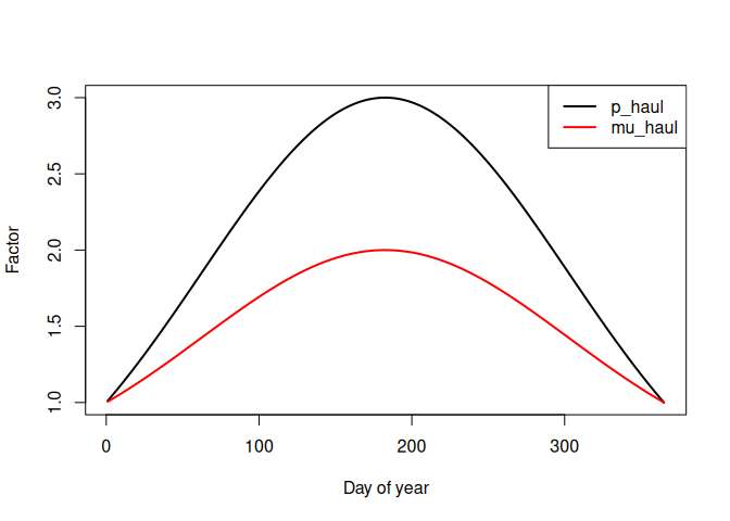
p_haul_max_multiplier <- 3 # haul rate can go up to Mx higher: here 3x i.e., 1 every 10 days
p_haul_doy_curve_sigma <- 120 # A fairly slow transition from max to min rate
p_haul_doy_curve <- dnorm(1:365, 182.5, p_haul_doy_curve_sigma)
p_haul_doy_curve <- scales::rescale(p_haul_doy_curve,c(1,p_haul_max_multiplier))
p_haul <- p_haul_base * p_haul_doy_curve

## Set up parameters for the total fish caught. We again make this greatest in
## winter, but it can only go up to 2x higher
mu_haul_base <- 600 # base mean haul
mu_haul_max_multiplier <- 2 # haul can go up to Mx higher
mu_haul_doy_curve_sigma <- 120
mu_haul_doy_curve <- dnorm(1:365, 182.5, mu_haul_doy_curve_sigma)
mu_haul_doy_curve <- scales::rescale(mu_haul_doy_curve,c(1,mu_haul_max_multiplier))
mu_haul <- mu_haul_base * mu_haul_doy_curve
Here’s what those multiplier curves look like:
Now let’s simulate those data by sampling from the two distributions (bernoulli and negative binomial).
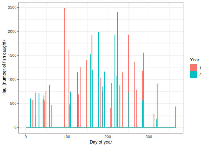
We’ll simulate 3 years of data, but use the first two for modelling and the 3rd for forecasting.
1
2
3
4
5
6
7
8
9
10
11
12
13
14
15
16
17
18
19
20
21
22
23
24
25
26
27
28
29
30
31
32
33
34
35
36
37
38
39
40
41
# Set the dispersion parameter *phi*. Lower is more overdispersed.
mu_haul_disp <- 5

N_years <- 3

d_sim_seasonal_frequency_3years <- tibble(
  time = 1:(365 * N_years),
  doy = rep(1:365, times = N_years),
  year = rep(c(1:N_years), each = 365),
  prob_haul = rep(p_haul, times = N_years),
  mean_haul = rep(mu_haul, times = N_years)
) %>%
  # we'll draw 1 sample per row. This is less efficient than passing a vector of
  # probabilities/means to rbinom and rnbinom (respectively) and then
  # multiplying the rnbinom samples by the rbinom samples, but it makes what
  # we're doing a lot more explicit
  # Here's what the code would look like if we did that
  ## mutate(
  ##  seasonal_haul_occ = rbinom(n(),1,prob_haul),
  ##  haul = seasonal_haul_occ*rnbinom(n(), size = mu_haul_disp, mu = mean_haul)
  ## )
  rowwise() %>%
  mutate(
    # Sample whether or not a haul occurs
    seasonal_haul_occ = rbinom(1, 1, prob_haul),
    haul = case_when(
      # if a haul occurred, sample its total
      seasonal_haul_occ == 1 ~ rnbinom(1, size = mu_haul_disp, mu = mean_haul),
      seasonal_haul_occ == 0 ~ 0
    )
  ) %>%
  ungroup() # turn off rowwise

d_sim_seasonal_frequency <- d_sim_seasonal_frequency_3years %>%
  filter(year < 3)

d_sim_seasonal_frequency %>%
  mutate(Year=as.factor(year)) %>%
  ggplot(aes(x=doy,y=haul,colour=Year,fill=Year))+
  geom_col()+
  labs(x= "Day of year",y="Haul (number of fish caught)")
Model the data!
We’ll use brms as it’s amazingly powerful and easy to use, it allows us to fit smooth curves via mgcv’s splines or gaussian processes, and it allows for distributional regression (i.e., we can model both the mean haul and the haul occurrence probability at once). Apart from that, it’s Bayesian, which is important in this case as we’ll use the posterior draws to make predictions and derive predicted cumulative haul, for which we want properly calibrated uncertainty estimates.
We’ll fit a model using cyclic splines by specifying bs="cc" in the smooth basis constructor call s(). Seven basis functions should be sufficient, as we don’t expect complicated wiggly curves for either the mean or hurdle components. There are alternatives, like Gaussian process smooths or a random-walk process built using a Markov Random Field (using mgcv’s mrf basis functionality alongside MRFtools). I’ve tested both and the GP was hard to fit while the MRF worked well but was a bit awkward to work with.
1
library(brms)
1
2
3
4
5
6
7
8
9
10
11
12
## Loading required package: Rcpp

## Loading 'brms' package (version 2.22.0). Useful instructions
## can be found by typing help('brms'). A more detailed introduction
## to the package is available through vignette('brms_overview').

##
## Attaching package: 'brms'

## The following object is masked from 'package:stats':
##
##     ar
1
2
3
4
5
6
7
8
9
10
11
12
13
14
15
16
17
18
19
m_hurdle_seasonal_haul_frequency <- brm(
  bf(
    # The haul varies throughout the year
    haul ~ s(doy, bs = "cc", k = 7),
    # ... and so does the probability of a haul (not) occurring (the "hurdle")
    hu ~ s(doy, bs = "cc", k = 7)
    ),
  knots = list(doy = c(1, 366)), # 1st of Jan = "32nd of Dec"
  family = hurdle_negbinomial(),
  data = d_sim_seasonal_frequency,
  cores = 4,
  refresh = 500,
  warmup = 1000,
  iter = 2000,
  control = list(adapt_delta = 0.995),
  backend = "cmdstanr",
  file = "m_hurdle_seasonal_haul_frequency"
)
m_hurdle_seasonal_haul_frequency
1
2
3
4
5
6
7
8
9
10
11
12
13
14
15
16
17
18
19
20
21
22
23
24
25
26
27
28
29
30
31
32
33
34
35
36
37
38
39
40
41
42
43
44
45
46
47
48
49
50
51
## Loading required package: rstan

## Loading required package: StanHeaders

##
## rstan version 2.32.7 (Stan version 2.32.2)

## For execution on a local, multicore CPU with excess RAM we recommend calling
## options(mc.cores = parallel::detectCores()).
## To avoid recompilation of unchanged Stan programs, we recommend calling
## rstan_options(auto_write = TRUE)
## For within-chain threading using `reduce_sum()` or `map_rect()` Stan functions,
## change `threads_per_chain` option:
## rstan_options(threads_per_chain = 1)

##
## Attaching package: 'rstan'

## The following object is masked from 'package:tidyr':
##
##     extract

## Warning: There were 1 divergent transitions after warmup. Increasing
## adapt_delta above 0.995 may help. See
## http://mc-stan.org/misc/warnings.html#divergent-transitions-after-warmup

##  Family: hurdle_negbinomial
##   Links: mu = log; shape = identity; hu = logit
## Formula: haul ~ s(doy, bs = "cc", k = 7)
##          hu ~ s(doy, bs = "cc", k = 7)
##    Data: d_sim_seasonal_frequency (Number of observations: 730)
##   Draws: 4 chains, each with iter = 2000; warmup = 1000; thin = 1;
##          total post-warmup draws = 4000
##
## Smoothing Spline Hyperparameters:
##                Estimate Est.Error l-95% CI u-95% CI Rhat Bulk_ESS Tail_ESS
## sds(sdoy_1)        0.20      0.13     0.06     0.54 1.00     1462     2198
## sds(hu_sdoy_1)     0.16      0.17     0.01     0.60 1.00     1279     1949
##
## Regression Coefficients:
##              Estimate Est.Error l-95% CI u-95% CI Rhat Bulk_ESS Tail_ESS
## Intercept        6.76      0.07     6.62     6.91 1.00     4898     3165
## hu_Intercept     2.67      0.15     2.39     2.98 1.00     4716     2654
##
## Further Distributional Parameters:
##       Estimate Est.Error l-95% CI u-95% CI Rhat Bulk_ESS Tail_ESS
## shape     4.30      0.87     2.76     6.19 1.00     3768     2409
##
## Draws were sampled using sample(hmc). For each parameter, Bulk_ESS
## and Tail_ESS are effective sample size measures, and Rhat is the potential
## scale reduction factor on split chains (at convergence, Rhat = 1).
The model takes about 30s to compile and samples very quickly and efficiently. Rhat and ESS look fine for all parameters.
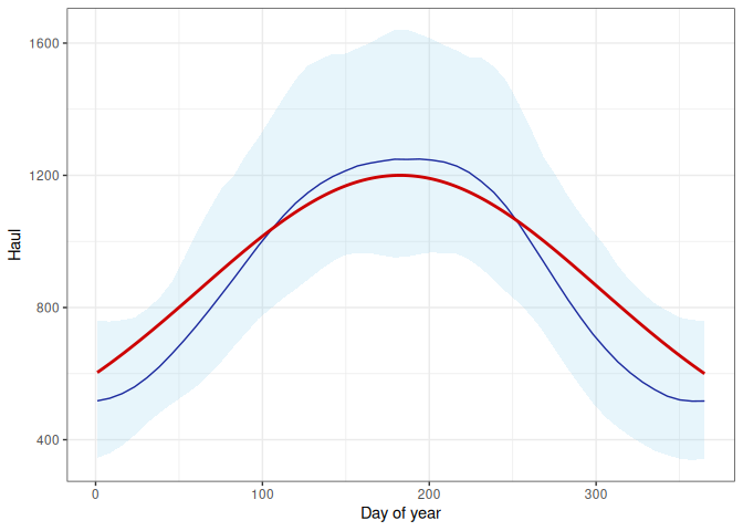
Let’s interrogate the model’s performance by checking that it reconstructs the expected change in haul and return probability over the year. I’ll use two different methods: marginaleffects::plot_predictions and brms::conditional_effects.
1
2
3
4
5
6
7
8
9
10
11
12
13
14
15
16
17
18
19
library(marginaleffects)

plot_predictions(m_hurdle_seasonal_haul_frequency,
                 condition = "doy",
                 type = "link",
                 draw = F) %>%
  mutate(across(c(estimate,conf.low,conf.high),exp)) %>%
  ggplot(aes(x=doy,y=estimate,ymin=conf.low,ymax=conf.high))+
  geom_line(colour="darkblue")+
  geom_ribbon(alpha=0.2,fill="skyblue")+
  geom_line(
    aes(x = doy, y = mean_haul),
    data = d_sim_seasonal_frequency %>%
      filter(year == 1),
    inherit.aes = F,
    colour="red3",
    linewidth=1
  )+
  labs(x="Day of year",y="Haul")
1
2
3
4
5
6
7
8
9
10
11
12
13
14
15
16
conditional_effects(
  m_hurdle_seasonal_haul_frequency,
  effects = "doy",
  dpar = "hu"
) %>%
  plot(plot = FALSE) %>%
  pluck(1) +
  geom_line(
    aes(x = doy, y = 1 - prob_haul),
    data = d_sim_seasonal_frequency %>%
      filter(year == 1),
    inherit.aes = F,
    colour = "red3",
    linewidth = 1
  )+
  labs(x="Day of year",y="Pr(No Haul)")
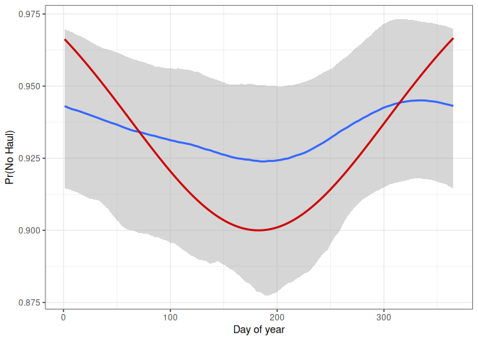
The model has done a good job identifying how haul size varies over the year, and a fair job with haul rate’s annual variation.
Predicting cumulative haul
Next, we want to see if we can derive cumulative haul predictions from our model, and check their accuracy.
Let’s make some convenience functions. We’ll also load tidybayes which comes with ggdist, and which we’ll use in the next section to conveniently generate forecasts.
1
library(tidybayes)
1
2
3
4
5
6
##
## Attaching package: 'tidybayes'

## The following objects are masked from 'package:brms':
##
##     dstudent_t, pstudent_t, qstudent_t, rstudent_t
1
2
3
4
5
6
7
8
9
10
11
12
13
14
15
16
17
18
19
20
21
22
23
24
25
26
27
28
29
30
31
32
predict_haul <- function(m, d) {
  predict(
    m,
    newdata = d,
    resp = "haul",
    summary = F,
    ndraws = 1000 # take 1000 draws from the model
  ) %>%
    as.data.frame() %>%
    rownames_to_column("drawid") %>%
    pivot_longer(-drawid, names_to = "time", values_to = "haul") %>%
    mutate(time = as.numeric(gsub("V", "", time))) %>%
    group_by(drawid) %>%
    # Cumulative sum of haul for each model draw
    mutate(cumulative_haul = cumsum(haul))
}

plot_cumulative_haul <- function(m, d, title) {
  out <- predict_haul(m, d) %>%
    ggplot(aes(x = time, y = cumulative_haul)) +
    geom_line(aes(group = drawid), alpha = .05) +
    stat_lineribbon(alpha = 0.4) +
    scale_fill_brewer() +
    geom_line(
      data = d %>%
        ungroup() %>%
        mutate(cumulative_haul = cumsum(haul)),
      colour = "red"
    ) +
    labs(title = title)
  return(out)
}
Now use them to plot the predictions alongside the data.
1
2
3
4
5
6
plot_hurdle_seasonal_haul_frequency_smooth<-plot_cumulative_haul(
  m_hurdle_seasonal_haul_frequency,
  d_sim_seasonal_frequency,
  "Seasonal haul and frequency -- Cyclic spline"
)
print(plot_hurdle_seasonal_haul_frequency_smooth)
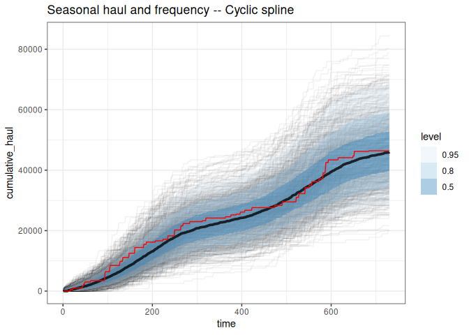
Looks decent! The true cumulative haul follows the predicted values nicely, and generally lies within the 50% credibility interval.
There is quite a lot of variance, though, but I think this is probably because we’ve deliberately simulated hard-to-predict data by using such an overdispersed negative binomial distribution, plus we only have two years of data. For example, take a look back at the model summary and note that the lower 95% CI estimate for the shape parameter was 2.76!
1
2
# Compare variances
var(rnbinom(5000,size=2.76,mu=600))
1
## [1] 129296
1
var(rnbinom(5000,size=4.30,mu=600))
1
## [1] 85057.88
1
var(rnbinom(5000,size=6.19,mu=600))
1
## [1] 57882.31
Our posterior draws can produce samples that differ greatly in variance.
Forecast
Remember that we actually simulated 3 years of data, but we only modelled the first two. This was so that we could check the model’s ability to forecast.
1
2
3
4
5
6
7
8
9
10
11
12
13
14
15
16
17
18
19
20
21
22
23
24
25
26
27
28
29
30
31
32
33
34
35
36
37
38
39
40
41
42
43
44
45
46
47
48
49
50
51
52
53
54
55
56
# Get the observed net haul at the end of year 2
cumulative_haul_end_year2 <- d_sim_seasonal_frequency_3years %>%
  filter(year != 3) %>%
  ungroup() %>%
  mutate(cumulative_haul = cumsum(haul)) %>%
  summarise(max_cumulative_haul = max(cumulative_haul)) %>%
  pluck("max_cumulative_haul")

pred_seasonal_year3_smooth <- d_sim_seasonal_frequency_3years %>%
  filter(year == 3) %>%
  select(-haul) %>%
  # Make predictions using tidybayes
  add_predicted_draws(
    m_hurdle_seasonal_haul_frequency,
    ndraws = 2000
  ) %>%
  rename(haul = .prediction) %>%
  # add in the observed haul for years 1 and 2
  bind_rows(
    d_sim_seasonal_frequency_3years %>%
      filter(year != 3),
    .
  ) %>%
  ungroup() %>% # NB!
  group_by(.draw) %>% # NB!
  # Calculate cumulative haul
  mutate(
    cumulative_haul = cumsum(haul),
    cumulative_haul = case_when(
      # if observed, take the actual value
      is.na(.draw) ~ cumulative_haul,
      # if predicted, start from the observed net haul after 2 years
      .draw > 0 ~ cumulative_haul + cumulative_haul_end_year2
    )
  )

### Plot ---
plot_pred_seasonal_year3_smooth <- pred_seasonal_year3_smooth %>%
  ggplot(aes(x = time, y = cumulative_haul)) +
  geom_line(aes(group = .draw), alpha = .05) +
  stat_lineribbon(
    alpha = 0.4,
    # it's crucial to only base this stat_ on predictions
    data = pred_seasonal_year3_smooth %>%
      filter(!is.na(.draw))
  ) +
  scale_fill_brewer() +
  geom_line(
    data = d_sim_seasonal_frequency_3years %>%
      ungroup() %>%
      mutate(cumulative_haul = cumsum(haul)),
    colour = "red"
  ) +
  labs(title = "Forecast -- Cyclic spline")

print(plot_pred_seasonal_year3_smooth)
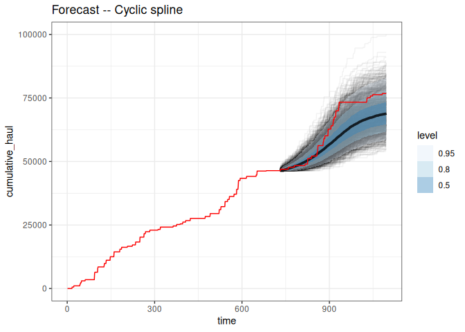
Conclusion
Overall, this approach seems reasonable to me, and given real data it could immediately be improved by including covariates, more informative priors, or just more years of data. If we had several vessels, variation among them could be incorporated using, for example, factor smooths (see ?mgcv::factor.smooth) or (maybe) 2d Markov Random Fields (see e.g., https://ecogambler.netlify.app/blog/phylogenetic-smooths-mgcv/; the phylogenetic effect would just be swapped out with a factor MRF for vessel).
Additionally, this simulation doesn’t prevent unusually short trips; e.g. at their most frequent, the probability of a haul is 1 every 10 days, but that doesn’t prevent two hauls from occurring sequentially.
To generate a more realistic data set, I was thinking we’d need to add time-dependent latency to the observations. In other words, we’d have a two-state Markov Model with states “at sea” and “haul”. This would add a transition probability matrix to the current model, which might look like this for simulation:
| to\from | at sea | haul |
|---|---|---|
| at sea | 0.9 | 1 |
| haul | 0.1 | 0 |
The probability of going from (columns) at sea to (rows) at sea is the probability of remaining at sea, and so on.
But after having written this out, I’m not so sure it makes sense. I need to think more about it, and perhaps I’ll follow up with another post.
That’s it for this nonsense!
1
sessionInfo()
1
2
3
4
5
6
7
8
9
10
11
12
13
14
15
16
17
18
19
20
21
22
23
24
25
26
27
28
29
30
31
32
33
34
35
36
37
38
39
40
41
42
43
44
45
46
47
48
49
50
51
52
53
54
55
56
57
58
## R version 4.4.2 (2024-10-31)
## Platform: x86_64-pc-linux-gnu
## Running under: Linux Mint 22.1
##
## Matrix products: default
## BLAS:   /usr/lib/x86_64-linux-gnu/blas/libblas.so.3.12.0
## LAPACK: /usr/lib/x86_64-linux-gnu/lapack/liblapack.so.3.12.0
##
## locale:
##  [1] LC_CTYPE=en_ZA.UTF-8       LC_NUMERIC=C
##  [3] LC_TIME=en_ZA.UTF-8        LC_COLLATE=en_ZA.UTF-8
##  [5] LC_MONETARY=en_ZA.UTF-8    LC_MESSAGES=en_ZA.UTF-8
##  [7] LC_PAPER=en_ZA.UTF-8       LC_NAME=C
##  [9] LC_ADDRESS=C               LC_TELEPHONE=C
## [11] LC_MEASUREMENT=en_ZA.UTF-8 LC_IDENTIFICATION=C
##
## time zone: Africa/Johannesburg
## tzcode source: system (glibc)
##
## attached base packages:
## [1] stats     graphics  grDevices datasets  utils     methods   base
##
## other attached packages:
##  [1] tidybayes_3.0.7        marginaleffects_0.25.1 rstan_2.32.7
##  [4] StanHeaders_2.32.10    brms_2.22.0            Rcpp_1.0.14
##  [7] lubridate_1.9.4        forcats_1.0.0          stringr_1.5.1
## [10] dplyr_1.1.4            purrr_1.0.4            readr_2.1.5
## [13] tidyr_1.3.1            tibble_3.2.1           ggplot2_3.5.2
## [16] tidyverse_2.0.0
##
## loaded via a namespace (and not attached):
##  [1] svUnit_1.0.6         tidyselect_1.2.1     farver_2.1.2
##  [4] loo_2.8.0            fastmap_1.2.0        tensorA_0.36.2.1
##  [7] digest_0.6.37        estimability_1.5.1   timechange_0.3.0
## [10] lifecycle_1.0.4      processx_3.8.6       magrittr_2.0.3
## [13] posterior_1.6.1      compiler_4.4.2       rlang_1.1.6
## [16] tools_4.4.2          yaml_2.3.10          collapse_2.1.1
## [19] data.table_1.17.0    knitr_1.50           labeling_0.4.3
## [22] bridgesampling_1.1-2 pkgbuild_1.4.7       curl_6.2.2
## [25] plyr_1.8.9           RColorBrewer_1.1-3   cmdstanr_0.8.1.9000
## [28] abind_1.4-8          withr_3.0.2          grid_4.4.2
## [31] stats4_4.4.2         xtable_1.8-4         colorspace_2.1-1
## [34] inline_0.3.21        emmeans_1.11.0       scales_1.4.0
## [37] dichromat_2.0-0.1    insight_1.2.0        cli_3.6.5
## [40] mvtnorm_1.3-3        rmarkdown_2.29       generics_0.1.3
## [43] RcppParallel_5.1.10  rstudioapi_0.17.1    reshape2_1.4.4
## [46] tzdb_0.5.0           splines_4.4.2        bayesplot_1.12.0
## [49] parallel_4.4.2       matrixStats_1.5.0    vctrs_0.6.5
## [52] V8_6.0.3             Matrix_1.7-3         jsonlite_2.0.0
## [55] arrayhelpers_1.1-0   hms_1.1.3            ggdist_3.3.3
## [58] glue_1.8.0           codetools_0.2-20     ps_1.9.1
## [61] distributional_0.5.0 stringi_1.8.7        gtable_0.3.6
## [64] QuickJSR_1.7.0       bspm_0.5.7           pillar_1.10.2
## [67] htmltools_0.5.8.1    Brobdingnag_1.2-9    R6_2.6.1
## [70] evaluate_1.0.3       lattice_0.22-7       backports_1.5.0
## [73] rstantools_2.4.0     coda_0.19-4.1        gridExtra_2.3
## [76] nlme_3.1-168         checkmate_2.3.2      mgcv_1.9-3
## [79] xfun_0.52            pkgconfig_2.0.3